Introduction

This is an informal introduction to the Determinant Quantum Monte Carlo (DQMC) algorithm. It is capable of simulating so-called "strongly correlated" quantum systems at high temperatures. Strongly correlated means that the quantum particles (typically electrons) cannot be well described by independent-electron approximations (like density functional theory or band structure calculations); a famous example are high-$T_c$ "cuprate" superconductors.

To get off the ground, we first need a model of the physical system. You have probably heard of the Schrödinger equation in quantum mechanics. The deceptive apparent simplicity of the equation $ i \hbar \partial_t \Psi = H \Psi$ stands in stark contrast to the difficulty of actually solving it numerically, once the wavefunction $\Psi$ describes "many" (think 10 or more) electrons simultaneously.

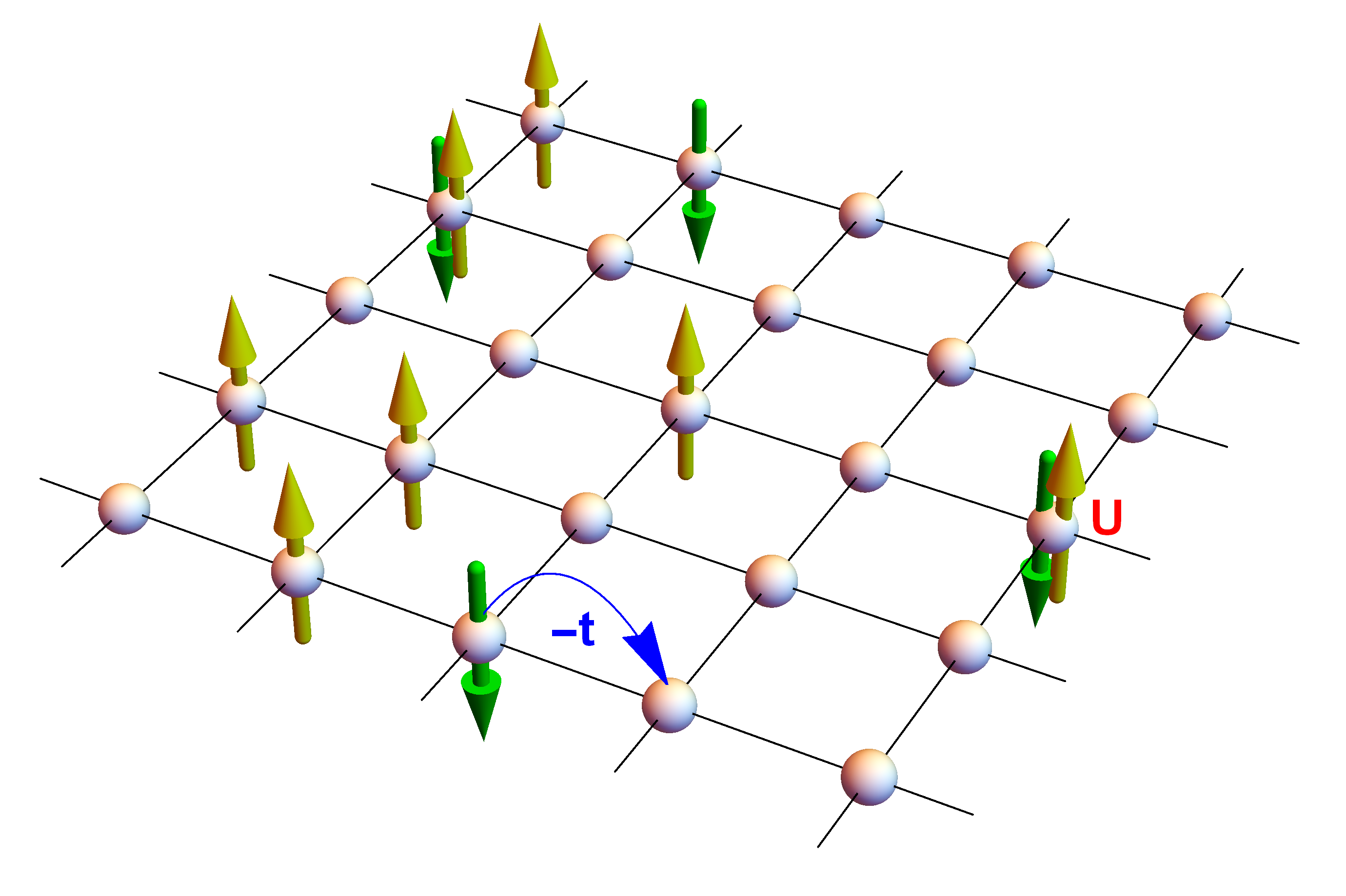
To simply matters a bit (pun intended), condensed matter theorists have come up with tight binding models as pictured above. Tell me more about tight binding models

Tight binding models are succinctly expressed in the languge of "second quantization". Specifically, the picture directly translates to the following Hamiltonian: \begin{equation} \label{eq:hubbard_hamiltonian} H = -{\color{blue}t} \sum_{\langle i,j \rangle, \sigma} \left(c^{\dagger}_{i\sigma} c_{j\sigma} + c^{\dagger}_{j\sigma} c_{i\sigma}\right) + {\color{red}U} \sum_i (n_{i\uparrow} - \tfrac{1}{2})(n_{i\downarrow} - \tfrac{1}{2}) \end{equation} The $c^{\dagger}_{i\sigma}$ and $c_{i\sigma}$ are the so-called fermionic creation and annihilation operators for lattice site $i$ and spin $\sigma$, and $n_{i\sigma} = c^{\dagger}_{i\sigma} c_{i\sigma}$. Informally, they add or remove an electron from lattice site $i$ with spin $\sigma$. The first term in \eqref{eq:hubbard_hamiltonian} (so-called kinetic hopping) precisely describes the hopping to neighboring lattice sites, while the second ("interaction") term penalizes double occupancy of a lattice site due to Coulomb repulsion.

Traces in quantum Fock-space

For a Hamiltonian of quadratic form $$ H = \sum_{i,j} {\color{blue}h}_{ij}\, c^{\dagger}_i c_j $$ the following exact identity holds: $$ \mathrm{tr}\big[\mathrm{e}^{-\beta H}\big] = \det\!\big[I + \mathrm{e}^{-\beta {\color{blue}h}}\big] $$ where $I$ is the identity matrix.

This is simple to check for a single "orbital", that is, for $H = \epsilon\, c^{\dagger} c$: $$ \mathrm{tr}\big[\mathrm{e}^{-\beta H}\big] = \langle 0 \vert \mathrm{e}^{-\beta \epsilon c^{\dagger} c} \vert 0 \rangle + \langle 1 \vert \mathrm{e}^{-\beta \epsilon c^{\dagger} c} \vert 1 \rangle = 1 + \mathrm{e}^{-\beta \epsilon}. $$ In the general case, consider a basis in which $\color{blue}h$ is diagonal.

Hubbard-Stratonovich transformation

However, Hubbard interaction term contains four-fermion operators … $\leadsto$ discrete Hubbard-Stratonovich transformation (using that $n_{i\sigma} \in \{0,1\}$, after Trotter splitting $\beta = \Delta\tau L$) $$ \mathrm{e}^{-\Delta\tau {\color{red}U} \sum_i (n_{i\uparrow} - \frac{1}{2})(n_{i\downarrow} - \frac{1}{2})} = \mathrm{e}^{-\Delta\tau {\color{red}U}/4}\, \tfrac{1}{2} \sum_{ {\color{forestgreen}s} = \pm 1} \mathrm{e}^{-\Delta\tau {\color{forestgreen}s} \lambda (n_{i\uparrow} - n_{i\downarrow})} $$ $\lambda$ determined by $\cosh(\Delta\tau \lambda) = \mathrm{e}^{\Delta\tau {\color{red}U}/2}$

From quantum ensemble averages to classical Monte Carlo

Applying Trotter splitting ($\beta = \Delta\tau L$) and the Hubbard-Stratonovich transformation eventually leads to $$ Z = \mathrm{tr}\!\left[\mathrm{e}^{-\beta H}\right] = \sum_{\{ {\color{forestgreen}s_{i\ell} } = \pm 1\}} \det\!\left[M^{\uparrow}({\color{forestgreen}s})\right] \det\!\left[M^{\downarrow}({\color{forestgreen}s})\right] $$ with $$ M^{\sigma}({\color{forestgreen}s}) = I + B^{\sigma}_{L-1}({\color{forestgreen}s})\,B^{\sigma}_{L-2}({\color{forestgreen}s}) \cdots B^{\sigma}_{0}({\color{forestgreen}s}), $$ where $$ B^{\sigma}_{\ell}({\color{forestgreen}s}) = \mathrm{e}^{\mp \Delta\tau \lambda {\color{blue}v}({\color{forestgreen}s_{\cdot \ell}})}\,\mathrm{e}^{-\Delta \tau k}, \quad \ell = 0, 1, \dots, L-1, $$ $k$ is the kinetic single-particle matrix and $$ {\color{blue}v}({\color{forestgreen}s_{\cdot \ell}}) = \begin{pmatrix} {\color{forestgreen}s_{1\ell}} & 0 & 0 & \dots \\ 0 & {\color{forestgreen}s_{2\ell}} & 0 & \dots \\ 0 & 0 & {\color{forestgreen}s_{3\ell}} & \dots \\ \vdots & \vdots & \vdots & \ddots \end{pmatrix}. $$

Determinant Quantum Monte Carlo

Introduction

Traces in quantum Fock-space

Hubbard-Stratonovich transformation

From quantum ensemble averages to classical Monte Carlo

More coming soon...